IB 2017 (EOS) Paper 3 HL

IB 2017 (EOS) Paper 3 HL

I found this a lovely example of the types of question,  I expect the College Board to gavitate toward in the future. Plus it is most helpful in your understanding of Economies of Scale (EOS).

(a)  Define the term Increasing Returns to Scale.

 

 

An increase in all inputs leads to a proportionally greater increase in output or, that an increase in all inputs by X% leads to a greater than X% increase in output.

 

 

 Increasing Returns are seen when output increases 1800 to 3000 (50% increase in inputs, while output increases by 60%)

(b)  Using the date in Table 1 to support your answer, identify how changes in inputs may result in constant returns to scale & in decreasing returns to scale.

 

Constant Returns are seen when output increases from 3000 to 4000 units (33% increase in inputs and output)

Decreasing Returns to Scale are seen if output increases from 4000 units – increase in inputs – 25%, while output increases by 20%.

 

Decreasing Returns to Scale are seen if output increases from 5000 units to 6000 units as inputs increase by 20%, while output increases by 14.6%.

 

Long-Run ATC Cheat Sheet (Economies of Scale)

Long-Run ATC Cheat Sheet 

(Economies of Scale)

Tentative

2012 Multiple Choice (LRS/EOS)

2012 Multiple Choice (LRS/EOS)

Answer - (A) an increase in demand will cause no change in the long-run equilibrium price.

Understand that constant cost industries in long-run equilibrium are producing at the bottom of their SRATC and LRATC curves. They are productively and allocatively efficient. Firms can enter and exit and the price of the good will not be affected. The LRS (long-run supply) curve is horizontal or perfectly elastic. When demand increases then the industry supply will adjust in exact proportion to the increase in demand. Long-Run price returns to the original price.

LRS/EOS Cheat Sheet here.

Answer - (B) downward sloping

Long-Run Average Total Costs must be falling as when inputs are added output is larger proportionally than the inputs. Costs are falling as we add inputs. The LRS curve is downward sloping as the firm has economies of scale. (It needs to expand) - Demand increases and industry supply increases proportionally more than the change in demand as resource prices fall due to Economies of Scale. We are on the downward sloping section of our LRATC curve. 

Answer - (D) a higher short-run price for gadgets, followed by an increase in the quantity produced.

Understand that this question is asking the same thing as #10 above,

 but it is referring to short-run affects.

IN the short-run as population increases (demand determinate) demand increases causing prices to rise,,, and in the short term firms respond by increasing the amount of labor they have to take advantage of the higher price to make profits.

More labor is hired, MC's increase as more labor is hired until the firm reaches profit max (MR=MC)

In the long run firms will enter (chasing profits) and the competition will force prices back to the original long-run equilibrium price. Why? the original price? It's a constant cost industry.

Answer - (C) It's long-run average total costs will fall.

Understand that this question is the same as #22. If the firm is experiencing EOS its Long-Run ATC curve is downward sloping,, 

(meaning that they are producing on the LRATC where it is downward sloping)

Of course it can only do this in the long-run as capital can only be added and firms can only enter in the long-run. As it adds more capital or expands its total costs will fall (its LRATC's will fall) as we can se form the above graph.

Do you get it??????

Diminishing Returns vs. Economies of Scale

Diminishing Returns vs. Economies of Scale

DMR (Short-Run effect) - adding more inputs(labor) to a fixed factor of production(factory) will lead to increasing output but eventually as more inputs are added output will decrease and eventually become negative.

We understand this as we have graphed it quite a bit.

As we add our initial amounts of labor the marginal product (the output attributed to the next worker hired) increases as workers are more efficient (able to specialize) at their work. Adding more and more workers will increase the the TP (total product) output but at a decreasing rate. If we are foolish and keep adding workers the amount of output will eventually start to decrease and eventually become negative.

Understand that the MC curve is the cost of Labor and the MC curve above the AVC curve is the firms supply curve.

D = P = MR = AR

Short-run Adjustments (firm)

If MR > MC we should hire more workers (increase output)

if MR < MC then we should fire some workers (decrease output)

If MR = MC then we are at profit max,, optimal quantity of workers.

In the Short-Run the firm can only adjust its amount of labor (output). 

We adjust our amount of output (quantity) to maximise profit (MR=MC). This of course changes as the price of the good increases or decreases. As the (price of the good) increases we can make more profit and therefore hire more labor.

We adjust our labor to the profit maximising point where MRP=MRC, this is from the resource costs section of the course. (Usually taught at the end of the course)

Understand that the Max profit point is where MR=MC and where MRP=MRC,,,, if there was a quantity of labor that would create more profit then we wouldn't be at profit max. 

So if we are at MR =MC, then we must be where MRP=MRC.

If MRP > MRC we should hire more workers (increase output)

if MRP < MRC then we should fire some workers (decrease output)

If MRP = MRC then we are at profit max,, optimal quantity of workers.

Conclusion - In the short-run the firm must choose the optimal amount of labor to reach profit max (The firm and society in general is constrained by diminishing marginal returns) 

EOS - (Long-Run Effect) - Competitive advantages gained by a firm that expands its size. These include efficiencies such as buying in bulk and therefore reducing unit costs or having one human resource department shared between factories.

Adjustments - enter/exit of firms, increase or decrease of firm size

In essence, EOS depends on the size of firms that can fit into an industry. If demand for the good increases and as firms rush into the industry and our firm grows larger and resource costs still fall then we say the firm has economies of scale (EOS). The industry can handle more firms and existing firms should increase their size. The firms LRATC's are falling as they produce more output(quantity).

If the firm becomes to large and loses efficiency due to being to large, then diseconomies of scale will occur. 

If the industry has the right amount of efficiency and size then we will say that the industry is a constant cost industry and resource prices are not affected by firms entering or exiting the industry.

Check out the LRS/LRATC curve cheat Sheet here.

(not quite finished)

Conclusion - depending on the industry's economies of scale - (constant, decreasing, increasing) 

If a company can achieve EOS then the company should expand (produce more)

If the firm's to big increasing costs then they should reduce their size (produce less)

If a firm is of an efficient size (in a constant cost industry) the they are at productively and allocatively efficient. The firm is producing at the minimum of the SRATC and the LRATC curve.

2009 B Microeconomics FRQ #1

2009 B Microeconomics FRQ #1

Watch me anser it here

https://youtu.be/yadprxzZMXo

(A) Draw a CLG for Mary & Company and show each of the following.

(i) The profit max output and price, labelled as Qm & Pm respectively.

(ii) The area of loss shaded completely.

(B) What must be true in the short run for the company to continue at a loss?

Memorise this phrase, " In order for a company to continue operation at a loss it must be covering its variable costs (labor). You will see this again.

(C) Assume now that the demand for cleaning products increases and that the company is not earning short-run economic profits. relative to this short-run situation, how does each of the following change in the long-run.

(i) The number of firms.

Increase - In the long-run more firms will enter the market as profits attract firms.

(ii) The company's profit.

Decrease - In the long run the firm will be in long-run equilibrium making zero economic profit.

(D) In the long-run if the company continues to produce, will it produce the allocatively efficient level of output? Explain.

Remember that the industry is a monopolistically competitive industry, 

In the long-run the allocatively efficient level of output will not be produced. 

Monopolistic Competition Cheat Sheet is here.

(E) In  the long-run will the company be operating in the region where 

economies of scales (EOS) exist.

Absolutely - 

First, You must know what economies of scales looks like. Economies of Scale is the left half of the LRATC curve. It means that even though quantity in the industry is increasing costs for those resources are falling. 

EOS post is here.

Now, look closely at the graph you were to have drawn and notice 

Even when the firm is in long-run equilibrium it will still be operating in the downward sloping section of the ATC and therefore in the EOS region.

2016 Microeconomics FRQ #3

You should have been able to recognise that the business above is in a monopolistically competitive market - differentiated products, no barriers to entry.

(A) Draw a CLG showing Camden's demand curve, marginal revenue curve, marginal cost curve, and long-run average total cost curve. Label Camden's profit maximising output Qm & Pm.

(B) On your graph in part (a) label the output at which total revenue is maximised QR.

Max revenue is where MR = 0, at that quantity revenue is maximised.

(C) Do firms in this market experience economies of scale, diseconomies of scale, or neither in long-run equilibrium? Explain.

College Board! "YOU SICK BASTARD"!

Refer back to the EOS - Economies of Scale post

Notice that where MR=MC intersect and we find our price and quantity the LRATC curve is sloping downward. This is the section of the LRATC (long run average total cost curve) where resource prices are decreasing in the industry. It's a decreasing cost industry or an increasing returns industry or this industry is experiencing economies of scale.

Economies of Scale (EOS) (Increasing, decreasing and constant) Cost Industries

Economies of Scale

Economies of scale can be classified into two main types: Internal – arising from within the company; and External – arising from extraneous factors such as industry size.

Internal has to do with efficiencies stemming from the fact that the company has become larger. Example: Due to the company now printing 10,000 flyers for their new product, cost per flyer has decreased. Companies tend to be able to negotiate lower prices for larger bulk orders. The lower costs push the short-run average total cost curves down and to the right.

External economies of scale have more to do with broad changes in the industry. Example: the introduction of computers into the business world have lowered costs for all businesses that choose to accept them.

The AP tends to ask questions about EOS in the multiple choice section and the FRQ section but they are looking for different aspects of the same thing.

I've tried to create a graphic to help explain EOS. Let's see if it can help.

First, lets look at the MC questions:

Answer - B The firm doubles its inputs and and output triples

If we look at the graph above we see EOS and increasing returns to scale on the left side of the long-run average total cost curve. Costs (EOS) are falling as output increases due to efficiencies. The doubling of inputs and output tripling is an example of increasing returns.

EOS or increasing returns to scale.

EOS tend to have to do with  a firm's costs while returns to scale have to do with addition of inputs and outputs in the long-run. They of course are closely related. I would say that the above question is a more increasing returns to scale question but I don't write the questions. Know that the AP exam relates the two as closely connected.

First Multiple Choice

Answer - E Long-run average total cost decrease as output increases

Again, by looking at the graphic above we see the LRATC curve is showing decreasing costs as output increases.

Economies of Scale has to due with long-run changes in the scale of production.

Answer - Diseconomies of scale

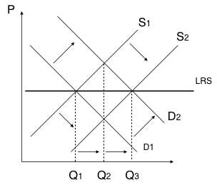
Answer - (a) The price will remain unchanged

(Demand increases and supply responds by increasing and pushing price back down to the original price)

The graphic above shows the differing ways that the sections can be referred to on the AP exam. 

Second FRQ's

The FRQ section of the AP gives you a guide when in the initial section of the question they speak about (Increasing cost industry -Decreasing cost industry - Constant cost industry) This is a warning that the LRATC curve will be discussed and you will be required to evaluate what happens to prices in the industry due to where the firm is on its  LRATC curve.

2015 Microeconomics  question #1

A constant-cost industry???? 

So in this question the firm is earning a positive profit, and profits attract other firms (firms enter) and supply increases which pushes the price lower.

The question would/could be how much lower as in lower than the original price, higher than the original price or equal to the original price.

In a constant cost industry supply will increase until the price is equal to the original price.

Example: 

So initially something happens in the short-run in the market, Demand increases. (D1 to D2)

This causes profits in the industry, profits firms enter, firms enter and supply increases (S1 to S2)

Supply increases to the original price. If a line is drawn between the original and the new equilibrium points we would get a horizontal line, this line is the Long Run supply curve.

2011B Microeconomics #1

Increasing Costs Industry - the firm is operating on the right side of the LRATC curve.

Here is what happens:

(C) Demand shifts right - price increases - causing profits - 

(D) (i) Profits attract firms (more firms) - supply increases - pushing down the price

Here is the important part::::

(ii) The firm's Short-run average total cost curve shifts up -  it is an increasing cost industry - costs are increasing - 

(i) Price has increased more than Pf.

(ii) Price is less than Pf2

If we look closely, we see that in an increasing costs industry, supply increases but not enough to lower price back to the original price. 

2008 Microeconomics #1

Constant Cost industry *****

So, Perfectly Competitive, Constant Cost in Long-run equilibrium

(b) Lump sum is given, which creates profits for the firm in the short-run

(iii) Number of firms can't change in the short-run,, tricky

(c) Indicate how changes in the Long Run

(i) Number of firms in the industry (Profits - firms enter - increases)

(ii) Price - Price will return back to the original price (price falls)

(iii) Industry Output 

(Demand increases and supply increase, price returns back to original price as it is a constant cost industry) Output in the industry increases