Perfect Competition (Long Run Supply/ATC Curves)

Perfect Competition (Long Run Supply/ATC Curves)

This stuff seems to give students crazy hard time. (because its complicated)

(see a problem drop me a line (wcwaugh@aol.com))

Creating this to mimic the AP College Boards FRQ's

1) Perfectly Competitive firm in long run equilibrium in a constant cost industry.

a) Demand increases (Price and quantity increases)

b) Firm makes profits (show) in SR

c) In the LR firms enter pushing supply back to original price.

d) Long Run supply curve is horizontal (firms enter but price of good doesn't change)

e) In a constant cost industry the firm is allocative and productively efficient

So, most FRQ's start with the firm in Long-Run Equilibrium and then market demand increasing/decreasing. The College Board asks you to show the effect of the market demand, profits/losses. 

Easy up to this point, Yes?

Then they ask you to explain what happens to the long run supply curve and what happens to the price in the market (compared to the original price).

Know that the Long Run Supply curve is simply a line drawn between the original equilibrium point and the equilibrium point after all firms have entered/exited the market. It shows the quantity supplied once producers have had time (long run) to enter/exit the industry.

Sometimes its easier to see the big picture or the flow of things. 

In essence the market is in equilibrium, no firms want to enter or exit as the existing firms are all making a normal profit. 

This implies that no adjustments need to be made.

No adjustments in the short-run (no labor needs to be hired or fired) and,

No adjustments in the long run (no firms entering or exiting the industry) 

then something happens (Demand increases) Why??? Look back at the Demand Supply Cheat Sheet!

Lets just say population increases,, so demand increases. (profits happen for firms)

These firms adjust in the short-run by hiring more labor.

Due to diminishing marginal returns firms might need to buy a larger factory and/or more machinery.

In the long-run (remember?) firms can enter/exit but also more capital can be added (factories and machinery) for firms that need to expand.

Supply increases but in this instance, supply increases proportionately more than demand had increased.

This is due to resource prices used in production decreasing marginally due to economies of scale.

More supply pushes the price of the good lower than the original price,, this happens again and again 

How does this look over time.

 Notice that demand increases but less than the supply curve increases. Prices are falling as firms get larger due to economies of scale. Think agriculture. At the turn of the last century in the US, 80% of the people worked on farms now the percentage is around 2%. Firms got more productive and much larger.

Food costs have fallen due to technology and the industry adjusted with different levels of labor/capital mixes.

What if we draw in the ATC curves in the short run. Here is the same graph above with the short-run atc curves drawn.

Understand that at each ATC curve is a point in time where the firm is back to equilibrium (normal profit) and has no reason to enter or exit. Then demand changes and firms scramble to supply more goods/services. As they hire more labor with the existing machinery/factories their costs rise and they decide to increase factory size. This increasing of factory/machinery lowers ((((marginal costs)))

Mr. Waugh, where is the Long-Run Supply Curve

Draw a line through all of the Long-Run Equilibrium points and you have your  Long-Run Supply Curve

Understand that in this decreasing cost industry, as demand increase, supply responds in ways that price falls in the market due to ATCs falling for the firm. 

There are connections to this graph.

In the above Firm graph,, if we are producing where MR>MC then we should produce more. How? Hire more people...   If we are producing where MC>MR then we should produce less. How?? Fire some people. We want to produce where MR=MC = Profit Max. This is the quantity society wants MC=MB from societies standpoint.

Now lets look at the Long-Run ATC curve with LRMR and LRMC

Left Side, a short run ATC and MC curve on a LRATC curve,, the Firm in the short run needs to increase in size, or more firms need to enter as costs can be driven down because of EOS.. More will be produced and society will pay for it. (((Assuming that the Demand increases)))

Right Side, this industry has to many firms or its firms are to large and costs are rising. Firms are to large or there are to many firms.

Middle - Constant cost industry, firms enter and exit without price changes. This is approximately the right amount of firms in this industry at this point.

Monopolistic Competition Cheat Sheet (Updated 01/04/2017)

Monopolistic Competition Cheat Sheet (Updated 01/04/2017)
Need a copy? E-mail wcwaugh@aol.com

2010 B Micro FRQ #1

2010 B Micro FRQ #1

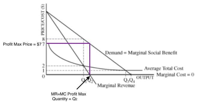
(A) Assume that the private firm owns the bridge and maximises profits. Determine the output and price.

This is why we learn the MR=MC rule and apply it to all maximising profit companies. Look for MR=MC and follow the lines, even when the college board thinks up a strange question like this.

(B) Now assume that a municipality owns the bridge and sets the price to achieve allocative efficiency . Determine the output and price.

From the Monopoly Cheat Sheet here.

Recognise and understand that Allocative Efficiency is where P = MC.

(C) At a price of $1, is the municipality's accounting profit positive, negative or zero? Explain.

Understand Accounting Profit: Profit Cheat Sheet Here.

Remember that Zero Economic Profit is positive accounting profit. At a price of $1, P = ATC.

This is a fair return or break-even price the monopolist will be making a normal or zero economic profit.

(D) Suppose the municipality sets a break-even price that generates revenue just to cover all economic costs.

(i) Based on the graph, determine break-even output.

(ii) At the output you determined in part (D)(i), is the demand relatively elastic, relatively inelastic, perfectly elastic, or perfectly inelastic or unit elastic.

(E) If a company provides access to the island via watercraft, what will happen to each of the following?

(i) The demand curve for bridge crossing.

Substitution causes the demand curve to shift to the left.

(ii) The profit maximising output.

If demand falls then output necessarily falls.

(F) Suppose the long-run average total cost curve is strictly downward sloping, would it be efficient to build a second bridge? Explain.

I have no problem stating that this problem is poorly worded and stumped quite a number of teachers of economics. Along with myself.

Take a step back and think about what you know:

1) The demand for this good is inelastic
2) Fair Return/ Break-Even price is $1
3) A competing water taxi will reduce demand for our bridge#1
4) The socially optimal quantity (SOQ) is 4 autos at a price of zero
5) To get more people to cross our bridge you would have to pay them - also inefficient
6) Building bridge #2 with a price of zero will just attract autos away from Bridge #1, & increase fixed costs and therefore Average Total Costs
7) This will raise Bridge #1's ATC's as the Demand curve for Bridge #1 shifts leftward.
8) Overall the municipality's ATC's will increase = inefficiency

I think,,, that the clue here is the understanding that allocative efficiency (Socially Optimal Quantity) is produced at a quantity of Q4. with a price of zero. Remember that the quantity is the number of cars crossing the bridge during the day and at a price of zero,, 4 autos cross that bridge. This is what society values as it is the SOQ and allocatively efficient level of production ..

Saying it another way,,,, If with one bridge at a price of zero demand is met. Then if we build a second bridge, the demand curve for bridge #1 will shift leftward (substitute) and its ATC's increase.

Saying it another way,,, There is no demand for a second bridge as the first bridge serves the socially optimal quantity (4) without raising the price above zero... in essence, because they are in the economies of scale section of the LRATC curve there is no reason to increase fixed costs (build another bridge) as the costs are still falling with increased production,,,, There is no reason to increase our fixed costs (bridge #2) until we have the need or demand.

One more point,, Obviously we want to produce were our ATC curve is lowest and as we are experiencing economies of scale we want to produce more but this is only efficient if there is enough demand. There isn't enough Demand. If we build a second bridge our fixed costs will increase and therefore our ATC will increase. This would makes us less efficient.

Profits Cheat Sheet (Updated) 12/24/2016

Profits Cheat Sheet (Updated) 12/24/2016

Students in Malta crushing my blog.

Malta

Here is a shout out to all of the QSI students in Malta studying for the AP economics exams.

I'm sitting here in Columbia SC listening to the Bay Retro radio station in Malta. http://radio.garden/live/saint-julians/bay/

Marie Louise Coleiro Preca would like you to get a 5

If your studying AP Economics and want your picture added to this page,, send me a picture of yourself studying economics, draw a graph on a window, wall, book, floor and have it added.

Send pictures here  - wcwaugh@aol.com

2010 AP Microeconomics FRQ #1

2010 AP Microeconomics FRQ #1

watch me answer it here

https://youtu.be/UvPSKfqzl6Y

(A) Assume that Farmer Roy is making zero economic profit in the short-run. Draw a correctly labeled side by side graph for the corn market and for Farmer Roy and show each of the following.

(i) The equilibrium price and quantity for the corm market.

(ii) The equilibrium quantity for farmer Roy , labeled QF1.

(B) Is Farmer Roy's corn, is the demand perfectly elastic, perfectly inelastic, relatively elastic or relatively inelastic or unit elastic? Explain.

So, you must have recognised by this point that the MR curve is the Demand curve for a Perfectly Competitive industry. Therefore "putting your thinking cap on" the Demand for Farmer Roy's corn is perfectly elastic.

MORE IMPORTANT: is for you to understand why Farmer Roy doesn't raise his price? IF Farmer Roy raises his price, then there are thousands (theoretically) of other firms that would have a lower price and therefore Farmer Roy's revenues would fall to zero.

What if Farmer Roy decides to lower his price? (bit harder to conceptualize), If Farmer Roy can sell all he wants at the price of PM1, then how would lowering his price get him any benefit... again, he can sell all he wants at that price,, lowering his price will not increase sales.....

Perfect Competition Cheat Sheet Updated here.

(C) Corn can be used as the input in the production of ethanol. The demand for ethanol has significantly increased.

(i) Show on your graph in part (A), the effect on the increase in demand for ethanol on the market price and the quantity of corn in the short-run, labelling the equilibrium price and quantity.

(ii) Show on your graph in part (A), the increase in the demand for ethanol on Farmer Roy's quantity of corn in the short-run.

(iii) How does the average total cost for Farmer Roy at QF2, compare with PM2?

I dislike this question, as it seems to be confusing and doesn't really test your knowledge of economics. This question is simply asking where geographically the ATC is at in reference to the new price. The ATC curve was tangent at Pm1, zero economic profit was being earned but when the price rises to Pm2 the ATC is lower meaning that positive economic profits are being earned.

(D) Corn is also an input in the production of cereal. What is the effect of the increased demand for ethanol on the equilibrium price and quantity in the cereal market in the short-run? Explain.

 If there is an increase in the demand for ethanol then the demand for corn must increase. If the demand for corn increases then the price of corn must increase and therefore the price and quantity of cereals must increase as corn in an input for cereals. 

Perfect Competition Cheat Sheet Updated 12/20/2016

Perfect Competition Cheat Sheet Updated 12/20/2016

I added 2 small parts - Why? doesn't the perfectly competitive firm raise its price. (In the perfectly competitive market there are thousands of firms, each competing with each other, and all goods are the same (homogenous). If you raise your price then there are so many competitors that your customers will just buy from someone else... Yes, even if you raise the price by a penny.... This doesn't work as well in the real world,, but the AP exam isn't the real world)

- Why? doesn't the perfectly competitive firm lower its price? (In the perfectly competitive market the perfectly elastic MRDARP curve. Perfectly elastic demand implies that the firm can sell all it wants at the market price... I'm gonna write that again,, the firm can sell all it wants at the market price... Why would I ever lower my price if I can sell all I want,, everything I make,,, anything that I build at the higher price????

I added this because so many of the people I'm tutoring this year,, seem to miss these simple points.