2012 Multiple Choice Government Intervention (Price floors, ceilings, indirect tax)

2012 Multiple Choice Government Intervention (Price floors, ceilings, indirect tax)

Government Intervention cheat sheet here.

Answer - (B) A shortage of 6 billion gallons

Understand, that the biggest problems with these problems is knowing a ceiling from a floor.

say it,,,,,

Floors are high

Ceilings are low

say it again,,,,

Floors are high

Ceilings are low 

You might be tempted to say that the shortage is 4 billion gallons but understand that at the new (government controlled) price the Qd increases to 12b.

12b(Qd) - 6b(Qs) = 6b actually supplied

Answer - (D) Decrease   Decrease

Answer - (B) create a shortage of flashlights

If demand increases but supply does not, then shortages occur.

Producers will only supply more of a good if the price of the good increases

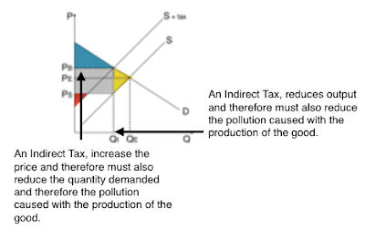
The NET price is the price received with the taxes taken out 

(amount the seller gets to put in his pocket)

18) Answer (D)

19) Answer (D)

Government Intervention Cheat Sheet Updated (01/12/2017)

Government Intervention Cheat Sheet Updated (01/12/2017)

Price Ceilings

Price Floors

Indirect Tax/Subsidy

Tariffs

2012 Oligopoly Multiple Choice

2012 Oligopoly Multiple Choice

Oligopoly Cheat Sheet here.

Answer - (A) Oligopoly

Understand that the word interdependence = oligopoly 

Answer - (C) A few competing sellers with similar products and high barriers to entry.

Recognise the definition of oligopoly?

Answer - (B) Both companies have an incentive to reduce production by 10%.

For the love of Pete, make a chart.

answer the chart.

Now, you know what they should do depending on the other (firms) actions,

but if they don't cooperate they don't know the other (firms) actions,

so, they don't cooperate.

Let us look at the answers 1 by 1

(A) Neither Company has a dominate strategy.

Actually both companies have dominate strategies UB (-10%) & UA (-20%)

Dominate Strategy - Best choice no matter the choice of the other participant. Doing the same thing no matter what the other firm does, is a dominate strategy.

Answer - (B) Both companies have an incentive to reduce production by 10%.

(B) is answered in the answer to (C), below

(C) Both companies have an incentive to reduce production by 20%

On first glance, this seems appropriate.

If they are both choosing to reduce by 20% then the payoffs would be $150 each, not bad.

but

this would only be true if they both new the information in the matrix

they don't

The problem says, based on the information, and assuming no cooperation,

assuming no cooperation implies they don't have information about the payoff matrix

so, if they don't know the information in the payoff matrix

they are going to choose the quadrant where they make the most money.

They do have the incentive of -20%, if they are cooperating

but they aren't cooperating.

The greedy principle....

Without knowing the information in the payoff matrix, they each choose the highest payoff

why not????

Because they both made the rational choice, highest payoff & didn't cooperate

they end up, making the least amount on the board.

(B) If the question had asked what the payoff would have been with no cooperation it

would have been 

UA chooses -10% and receives  $100

UB chooses -10% and receives  $100

This was the question and is the answer to (B)

(D) Only UA has an incentive to reduce production by 20%

We can look at the graph directly above,, and see that with the greedy principle, not knowing the payoff matrix, and not cooperating that UA would choose the highest daily payoff

of $250 which is in the -10% quadrant

(E) Only UA has an incentive to reduce production by 20%

Same reason as (D) above but with UB

We can look at the graph directly above,, and see that with the greedy principle, not knowing the payoff matrix, and not cooperating that UB would choose the highest daily payoff

of $250 which is in the -10% quadrant

COLLEGE BOARD

2012 (Resource Costs) Labor, Multiple Choice

2012 Multiple Choice (Resource Costs) Labor
Labor Cheat Sheet Here.

Answer #26 (B) 4

Make a chart as these questions are almost always set up the same way.

Whatever chart you use do it the same way every time.

Understand that we hire at Profit max for labor which is where MRP=MRC, or as close as we can get.

So we would hire the 4th workers as she brings in $50 (marginally) and we pay her $40 in a wage,, this gives us a $10 profit on her hire. We would not hire worker #5 as he only brings in $25 and we would have to pay him $40,, this hire would cost us $15... We lose money on  the 5th hire.

Answer #27 (A) 19

What is the MPP??

Understand that this is the same formula for the MP,,

 as the change in labor for all of these problems changes by one.

  

Answer - (A) The marginal product per dollar spent on labor is equal to the marginal product per dollar spent on capital.

Least-Cost Post here.

Answer - (B) Horizontal and downward sloping

Understand that this is a recognition problem, if it is a 

perfectly competitive market, Demand curve is the MRDARP curve 

and

the Firm's Labor demand curve is the MRP curve and it is downward sloping.

Answer - (D) MRP = MFC

Understand that sometimes the AP uses Marginal Factor Cost and sometimes Marginal Resource Cost as the wage rate.

same same

2012 Multiple Choice (LRS/EOS)

2012 Multiple Choice (LRS/EOS)

Answer - (A) an increase in demand will cause no change in the long-run equilibrium price.

Understand that constant cost industries in long-run equilibrium are producing at the bottom of their SRATC and LRATC curves. They are productively and allocatively efficient. Firms can enter and exit and the price of the good will not be affected. The LRS (long-run supply) curve is horizontal or perfectly elastic. When demand increases then the industry supply will adjust in exact proportion to the increase in demand. Long-Run price returns to the original price.

LRS/EOS Cheat Sheet here.

Answer - (B) downward sloping

Long-Run Average Total Costs must be falling as when inputs are added output is larger proportionally than the inputs. Costs are falling as we add inputs. The LRS curve is downward sloping as the firm has economies of scale. (It needs to expand) - Demand increases and industry supply increases proportionally more than the change in demand as resource prices fall due to Economies of Scale. We are on the downward sloping section of our LRATC curve. 

Answer - (D) a higher short-run price for gadgets, followed by an increase in the quantity produced.

Understand that this question is asking the same thing as #10 above,

 but it is referring to short-run affects.

IN the short-run as population increases (demand determinate) demand increases causing prices to rise,,, and in the short term firms respond by increasing the amount of labor they have to take advantage of the higher price to make profits.

More labor is hired, MC's increase as more labor is hired until the firm reaches profit max (MR=MC)

In the long run firms will enter (chasing profits) and the competition will force prices back to the original long-run equilibrium price. Why? the original price? It's a constant cost industry.

Answer - (C) It's long-run average total costs will fall.

Understand that this question is the same as #22. If the firm is experiencing EOS its Long-Run ATC curve is downward sloping,, 

(meaning that they are producing on the LRATC where it is downward sloping)

Of course it can only do this in the long-run as capital can only be added and firms can only enter in the long-run. As it adds more capital or expands its total costs will fall (its LRATC's will fall) as we can se form the above graph.

Do you get it??????

Diminishing Returns vs. Economies of Scale

Diminishing Returns vs. Economies of Scale

DMR (Short-Run effect) - adding more inputs(labor) to a fixed factor of production(factory) will lead to increasing output but eventually as more inputs are added output will decrease and eventually become negative.

We understand this as we have graphed it quite a bit.

As we add our initial amounts of labor the marginal product (the output attributed to the next worker hired) increases as workers are more efficient (able to specialize) at their work. Adding more and more workers will increase the the TP (total product) output but at a decreasing rate. If we are foolish and keep adding workers the amount of output will eventually start to decrease and eventually become negative.

Understand that the MC curve is the cost of Labor and the MC curve above the AVC curve is the firms supply curve.

D = P = MR = AR

Short-run Adjustments (firm)

If MR > MC we should hire more workers (increase output)

if MR < MC then we should fire some workers (decrease output)

If MR = MC then we are at profit max,, optimal quantity of workers.

In the Short-Run the firm can only adjust its amount of labor (output). 

We adjust our amount of output (quantity) to maximise profit (MR=MC). This of course changes as the price of the good increases or decreases. As the (price of the good) increases we can make more profit and therefore hire more labor.

We adjust our labor to the profit maximising point where MRP=MRC, this is from the resource costs section of the course. (Usually taught at the end of the course)

Understand that the Max profit point is where MR=MC and where MRP=MRC,,,, if there was a quantity of labor that would create more profit then we wouldn't be at profit max. 

So if we are at MR =MC, then we must be where MRP=MRC.

If MRP > MRC we should hire more workers (increase output)

if MRP < MRC then we should fire some workers (decrease output)

If MRP = MRC then we are at profit max,, optimal quantity of workers.

Conclusion - In the short-run the firm must choose the optimal amount of labor to reach profit max (The firm and society in general is constrained by diminishing marginal returns) 

EOS - (Long-Run Effect) - Competitive advantages gained by a firm that expands its size. These include efficiencies such as buying in bulk and therefore reducing unit costs or having one human resource department shared between factories.

Adjustments - enter/exit of firms, increase or decrease of firm size

In essence, EOS depends on the size of firms that can fit into an industry. If demand for the good increases and as firms rush into the industry and our firm grows larger and resource costs still fall then we say the firm has economies of scale (EOS). The industry can handle more firms and existing firms should increase their size. The firms LRATC's are falling as they produce more output(quantity).

If the firm becomes to large and loses efficiency due to being to large, then diseconomies of scale will occur. 

If the industry has the right amount of efficiency and size then we will say that the industry is a constant cost industry and resource prices are not affected by firms entering or exiting the industry.

Check out the LRS/LRATC curve cheat Sheet here.

(not quite finished)

Conclusion - depending on the industry's economies of scale - (constant, decreasing, increasing) 

If a company can achieve EOS then the company should expand (produce more)

If the firm's to big increasing costs then they should reduce their size (produce less)

If a firm is of an efficient size (in a constant cost industry) the they are at productively and allocatively efficient. The firm is producing at the minimum of the SRATC and the LRATC curve.