Monopolistic Competition

Monopolistic Competition

Assumptions

• many buyers and sellers
• heterogeneous/differentiated goods: (packaging, branding, after-sales service)
• low degree of price setting
• low barriers for entry and exit
• imperfect information

Monopolistic Competition, video - mjmfoodie

Revenue Curves

• Downward sloping demand curve
• Relatively, but not perfectly elastic, demand curve
• MR curve below Demand for same reason as monopoly

Profit Max in Short-run

• Firm produces at profit max
• Profits/losses possible in the short-run

Long-Run

• Entry/exit in the long-run will eliminated profits/losses
• Break-even only happens in the Long-run (like Perfect Competition)

Non-Price Competition

• Branding - development of recognizable brand in an attempt to develop brand loyalty
• Product Development - continuous improvement
• Customer Service - good service increases demand
• Location - convenient location increases demand
• Advertising - makes buyers aware of products

Efficiency

• Allocative Efficiency - (P = MC)
• Productively Efficient - (P = minATC)
• Monopolistic Competition neither achieves Allocative or Productive Efficiency

Monopolistic Competition compared to Perfect Competition

P (is higher)

Q (is lower)

Consumer Surplus (is less)

Allocative and Productive Efficiency (not achieved)

Product (differentiated)

Welker - Monopolistic Competition - Video

(Monopolistic Competition FRQ's 2009, 2007, 2004)

2009 AP Microeconomics Exam FRQ, Q1

Monopoly 9 - AP exam necessities

• Total Profit = (P-ATC) x Q
• Profit for 1 unit = (P-ATC) x 1
• TR = (P x Q) 
• Allocative Efficiency = (MC = D) or (P = MC) also called Socially Optimal Level/Quantity or Socially Efficient Quantity
• Marginal Revenue is negative = inelastic section of Demand curve.
• Marginal Revenue is  positive = elastic section of demand curve.
• Zero Economic Profit = (P = ATC)
• Positive Economic Profit = (P > ATC)
• Losses(P < ATC) 
• Profit Max = (MR = MC)
• Max Revenue = (MR = 0) where TR is maxed.
• Break-even = (P = ATC)
• Unit Elasticity = (MR = 0)
• Inelasticity = (MR < 0) or negative
• Elasticity = (MR > 0) or positive
• Demand curve is above MR, why? 
• Economic Profit = TR - explicit - implicit
• If you raise your price and TR (decreases) you are in the elastic section of Demand curve
• If you lower your price and TR (increases) you are in the elastic section of the Demand curve
• If you raise your price and TR (increases) you are in the inelastic section of the Demand curve
• If you lower your price and TR (decreases) you are in the inelastic section of the demand curve
• If demand shifts, what happens to P, Q, & MR?
• Positive Accounting Profits = (covering explicit costs)
• Opportunity Cost = implicit costs (implicit costs include entrepreneurs payment to self)
• (MC > P) = (MSC > MSB) = Society has enough units of this product (Overproduction)
• (P = MC) = Allocative Efficiency (MSB = MSC)
• (MC < P) = (MSB > MSC) = (P > MC) = Society values more of this product (Underproduction)
• Accounting Profit + Explicit Cost = Total Revenue
• Accounting profit - implicit costs = Economic Profit
• Economic Profit  = TR - explicit + implicit costs
• Accounting profit = TR - explicit costs
• Total Revenue - explicit costs = Accounting Profit
• Monopoly is the industry thus it has a downward sloping demand curve
• MR is less than Price(Demand) - for every level of output (except the first), why? - the lower price applies not only to the extra output sold but also to all prior units of output.

Monopoly 8 - Price Discrimination

Monopoly 8 - Price Discrimination

Price Discrimination Monopoly - Video - Welker

Price Discrimination -  exists when a producer charges a different price to consumers for an identical good or service.

Assumptions:

• the firm must possess some degree of market power (downward sloping demand curve)
• elasticity of demand is different in different markets
• firm must be able to separate markets with similar elasticities  to prevent reselling

Video of 1st, 2nd & 3rd degree

First degree 

First degree discrimination, known as perfect price discrimination, occurs when a firm charges a different price for every unit consumed.

The firm is able to charge the maximum possible price for each unit which enables the firm to capture all available consumer surplus for itself. In practice, first-degree discrimination is rare.

Second degree

Second-degree price discrimination means charging a different price for different quantities, such as quantity discounts for bulk purchases.

Third degree

Third-degree price discrimination means charging a different price to different consumer groups. For example, rail and tube travellers can be subdivided into commuter and casual travellers, and cinema goers can be subdivide into adults and children. Splitting the market into peak and off peak use is very common and occurs with gas, electricity, and telephone supply, as well as gym membership and parking charges. Third-degree discrimination is the commonest type.

Necessary conditions for successful discrimination

Graph - 

• More output
• More profit

Many pay higher prices, but some pay below the single price

2013 AP Microeconomics Exam

Monopoly 7 - Lump-Sum & Per-Unit

Monopoly 7 - Lump-Sum & Per-Unit

The AP exam will often ask you to correctly graph a monopoly firm's profits or loss and then evaluate what happens if a per-unit/lump-sum tax or subsidy is imposed/provided. 

You must know how to answer what happens to the firms, quantity, price, profits, consumer surplus, DWL, losses due to a per-unit or lump-sum.

Remember, a lump-sum is treated/viewed as a Fixed Cost (FC) and therefore will shift the ATC curve up(tax) or down (subsidy) but it will not effect the MC marginal cost curve.

*It appears that Subsidy and Tax are only asked/answered for short-run.  

Lump-Sum Subsidy - Monopoly 

Q- No change - (as MC not effected)

P - No change - (as MC not effected)

CS - No change - (as MC not effected)

DWL - No change - (as MC not effected)

Profits (increase) Losses (decrease)

Lump-Sum Tax - Monopoly

Q- No change - (as MC not effected)

P - No change - (as MC not effected)

CS - No change - (as MC not effected)

DWL - No change - (as MC not effected)

Profits (decrease) Losses (increase)

A per-unit tax is treated as a VC, variable cost and will shift the ATC up(tax) or down(subsidy) but it will also shift the MC curve left(tax) or right(subsidy).

Per-Unit Tax - Monopoly (graph to come)

Q - Decrease (MC will shift left and up)

P - Increase (MC will shift left and up)

CS - Decrease

Profits (decrease) Losses (increase)

DWL - Increase (less supplied DWL increases) “Quantity levels less than or greater than the efficient quantity create efficiency losses (or deadweight losses).”

Q is decreasing, price is increasing, profits (decrease) Losses (increase), DWL has increased as less is produced.

Per-Unit Subsidy - Monopoly (graph to come)

Q - Increase (MC will shift right and down)

P - Decrease (MC will shift right and down)

CS - Increase

Profits (increase) Losses (decrease)

DWL - Decrease (more supplied DWL decreases)  “Quantity levels less than or greater than the efficient quantity create efficiency losses (or deadweight losses).”

Q is increasing,  price is decreasing, profits (increase) Losses (decrease), DWL has decreased as less is produced.

Notice, the farther from Socially Efficient Quantity,, DWL increases. (anyone know something different, leave a comment)

 2012 AP Economics Exam FRQ, Q1

2007 AP Microeconomics Exam

Monopoly 6 Consumer/Producer Surplus & DWL

Monopoly 6 Consumer/Producer Surplus & DWL

Consumer/Producer Surplus

Notice that where Allocative efficiency occurs Consumer Surplus and Producer surplus is maximized.

2008 AP Microeconomics Exam

Answer (D)

As we know that Profit max is a higher price and a lower output,, and allocative efficient level has a lower price (good for consumers) and more output (good for consumers), then we know that consumer surplus has increased. Think of this problem by focusing on what has changed.

2008B AP Microeconomics Exam FRQ, Q1

2006 AP Microeconomics Exam FRQ, Q1

Look at (iii) The museum maximizes the consumer/producer surplus.

Notice that where Allocative efficiency occurs Consumer Surplus and Producer surplus is maximized.

Answer (P4, Q3), where P=MC

DWL (Dead Weight Loss)

Remember that a monopoly is a form of market failure, thus it has DWL.

Welfare Loss, or dead weight loss - refers to decreases in producer and/or consumer surplus as a result of either more or less than the socially optimal level of output produced and consumed.

2003 AP Microeconomics Exam FRQ, Q2

Look at (C)(ii) Deadweight loss

Monopoly - 5 Max Revenue & the Socially Efficient Quantity

Monopoly - 5 Max Revenue & the Socially Efficient Quantity

Some times a monopoly firm may choose to produce where revenue is maximized not profits. Why? In some situations managers might receive bonuses for sales, so we can expect them to act accordingly and sell where revenue is maximized. Notice, that when Max Rev is chosen that price is lower than Max Profit and more quantity is produced.

2008 AP Microeconomic Exam

Answer (C) P3/Q3

To max revenue, simply find where the MR curve crosses the bottom axis and draw a dotted line straight up until bumping into the demand curve and then turn left to get the rev max price. Do not assume that where MC crosses the Demand curve is automatically the Max Rev p/q,  as it is drawn like that quite often, but as we see above, not always.

2008B AP Microeconomics FRQ, Q1

Again, to find max revenue, simply find where the MR curve crosses the bottom axis and draw a dotted line straight up until bumping into the demand curve and then turn left to get the rev max price.

2004B AP Microeconomics Exam FRQ, Q1

Socially Efficient Quantity/Socially Optimal Level/Allocative Efficient Level

(The AP will/can use any of the above for where the MC curve meets the Demand Curve)

Notice, the SOQ/SEQ or allocative efficient level is below Max Rev/Profit and produces more output.

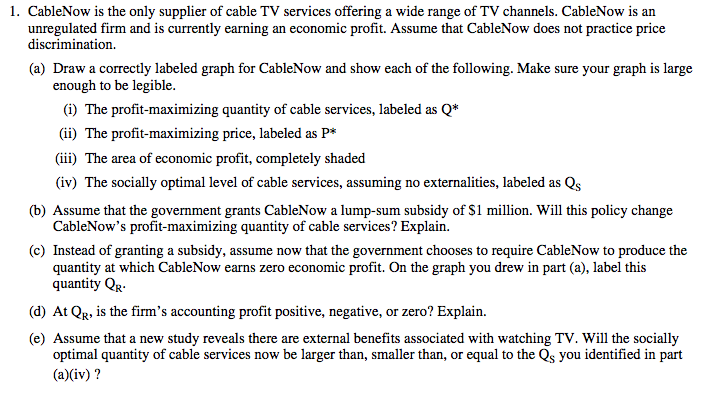
2013 AP Microeconomics Exam FRQ, Q1

MC = D, A monopoly firm would never choose to operate at this level.

2009 AP Microeconomics Exam, FRQ, Q1